Power Analysis for Two-Sample t-Tests: A Worked Example

A reproducible walkthrough of sample size and power calculations for two-sample t-tests, with simulated power curves across common effect sizes.

Introduction

Determining adequate sample size before data collection is a cornerstone of rigorous experimental design. The required sample size depends on the expected effect size, the desired power \((1 - \beta)\), and the significance level \(\alpha\). This post provides a reproducible walkthrough using R’s built-in power.t.test function.

We follow the framework of (Cohen 1988), which introduced the widely-used conventions for small (\(d = 0.2\)), medium (\(d = 0.5\)), and large (\(d = 0.8\)) effect sizes.

Sample size formula

For a balanced two-sample t-test, the minimum sample size per group is determined by:

\[ n = \frac{2\sigma^2(z_{1-\alpha/2} + z_{1-\beta})^2}{\delta^2} \]

where \(\delta\) is the true mean difference, \(\sigma^2\) is the common variance, \(z_{1-\alpha/2}\) is the critical value for a two-tailed test at level \(\alpha\), and \(z_{1-\beta}\) is the critical value for power \(1 - \beta\).

Setup

Power curves by effect size

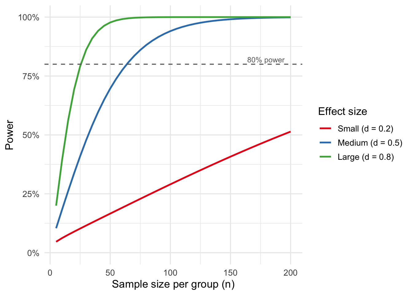
The plot below shows how statistical power changes as a function of sample size for three canonical effect sizes.

effect_sizes <- c(0.2, 0.5, 0.8)
n_seq <- seq(5, 200, by = 5)

power_grid <- expand.grid(n = n_seq, d = effect_sizes) |>
  rowwise() |>
  mutate(
    power = power.t.test(
      n = n, delta = d, sd = 1,
      sig.level = 0.05, type = "two.sample",
      alternative = "two.sided"
    )$power
  ) |>
  ungroup() |>
  mutate(effect = factor(d, labels = c("Small (d = 0.2)",
                                        "Medium (d = 0.5)",
                                        "Large (d = 0.8)")))

ggplot(power_grid, aes(x = n, y = power, color = effect)) +
  geom_line(linewidth = 1) +
  geom_hline(yintercept = 0.80, linetype = "dashed", color = "grey40") +
  annotate("text", x = 195, y = 0.82, label = "80% power",
           hjust = 1, size = 3.2, color = "grey40") +
  scale_y_continuous(labels = scales::percent_format(),
                     limits = c(0, 1)) +
  scale_color_brewer(palette = "Set1") +
  labs(x = "Sample size per group (n)",
       y = "Power",
       color = "Effect size") +
  theme_minimal(base_size = 13)

Figure 1: Power curves for a two-sample t-test (α = 0.05, two-tailed) across small (d = 0.2), medium (d = 0.5), and large (d = 0.8) Cohen’s d effect sizes.

Minimum n for 80% power

min_n_table <- tibble(
  `Effect size (d)` = c(0.2, 0.5, 0.8),
  Label = c("Small", "Medium", "Large")
) |>
  rowwise() |>
  mutate(
    `Min n per group` = ceiling(
      power.t.test(
        delta = `Effect size (d)`, sd = 1,
        sig.level = 0.05, power = 0.80,
        type = "two.sample", alternative = "two.sided"
      )$n
    )
  ) |>
  ungroup()

knitr::kable(min_n_table)

Table 1: Minimum sample size per group required to achieve 80% power at α = 0.05 (two-tailed two-sample t-test).

Effect size (d)	Label	Min n per group
0.2	Small	394
0.5	Medium	64
0.8	Large	26

Detecting a small effect (\(d = 0.2\)) requires substantially more participants than detecting a large effect — a practical reminder that underpowered studies are most likely to miss precisely the effects that are hardest to measure.

References

Cohen, Jacob. 1988. Statistical Power Analysis for the Behavioral Sciences. 2nd ed. Lawrence Erlbaum Associates.